


GWs from first-order phase transitions
David J. Weir, University of Helsinki
NORDITA, 5 July 2017
arXiv:1705.01783 and references therein
What's next? LISA

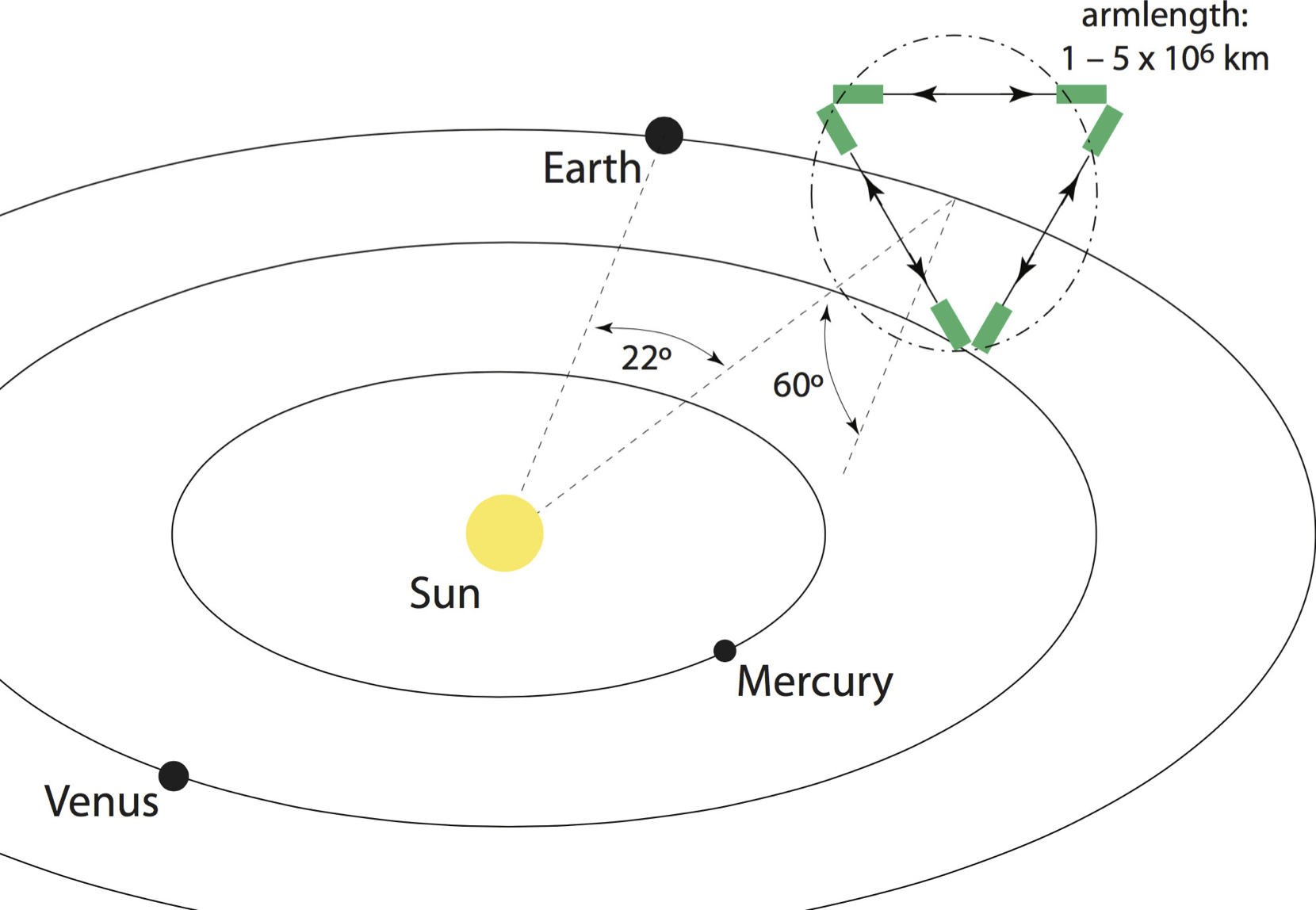
- LISA: three arms (six laser links), 2.5 M km separation
- Launch as ESA’s third large-scale mission (L3) in (or before) 2034
- Proposal officially submitted earlier this year arXiv:1702.00786
- Officially adopted on 20.6.2017
From the LISA proposal:
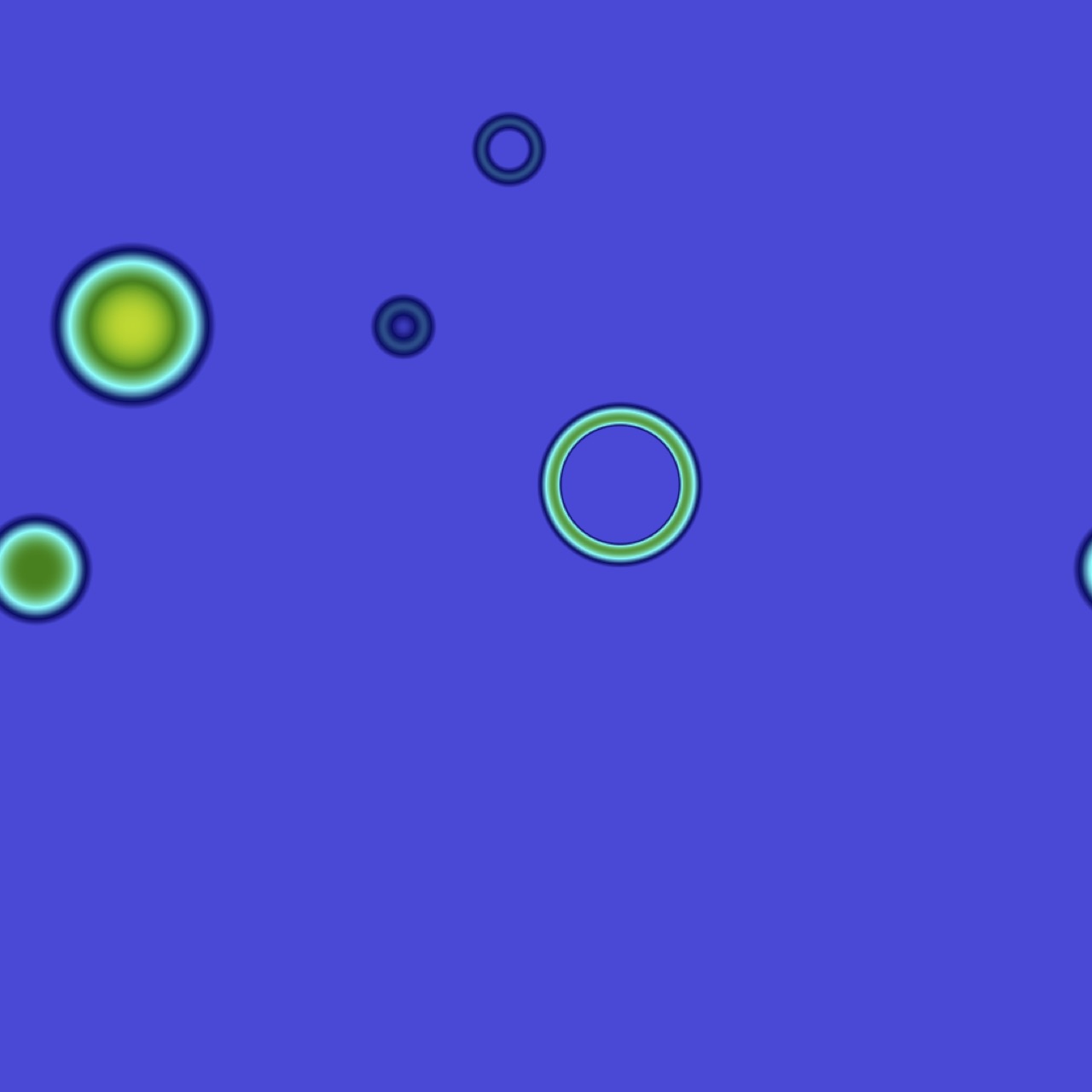
First order thermal phase transition:
- Bubbles nucleate and grow
- Expand in a plasma - create shock waves
- Bubbles + shocks collide - violent
process
- Sound waves left behind in plasma
- Turbulence; expansion
- Bubbles nucleate and grow
- Expand in a plasma - create shock waves
- Bubbles + shocks collide - violent process
- Sound waves left behind in plasma
- Turbulence; expansion
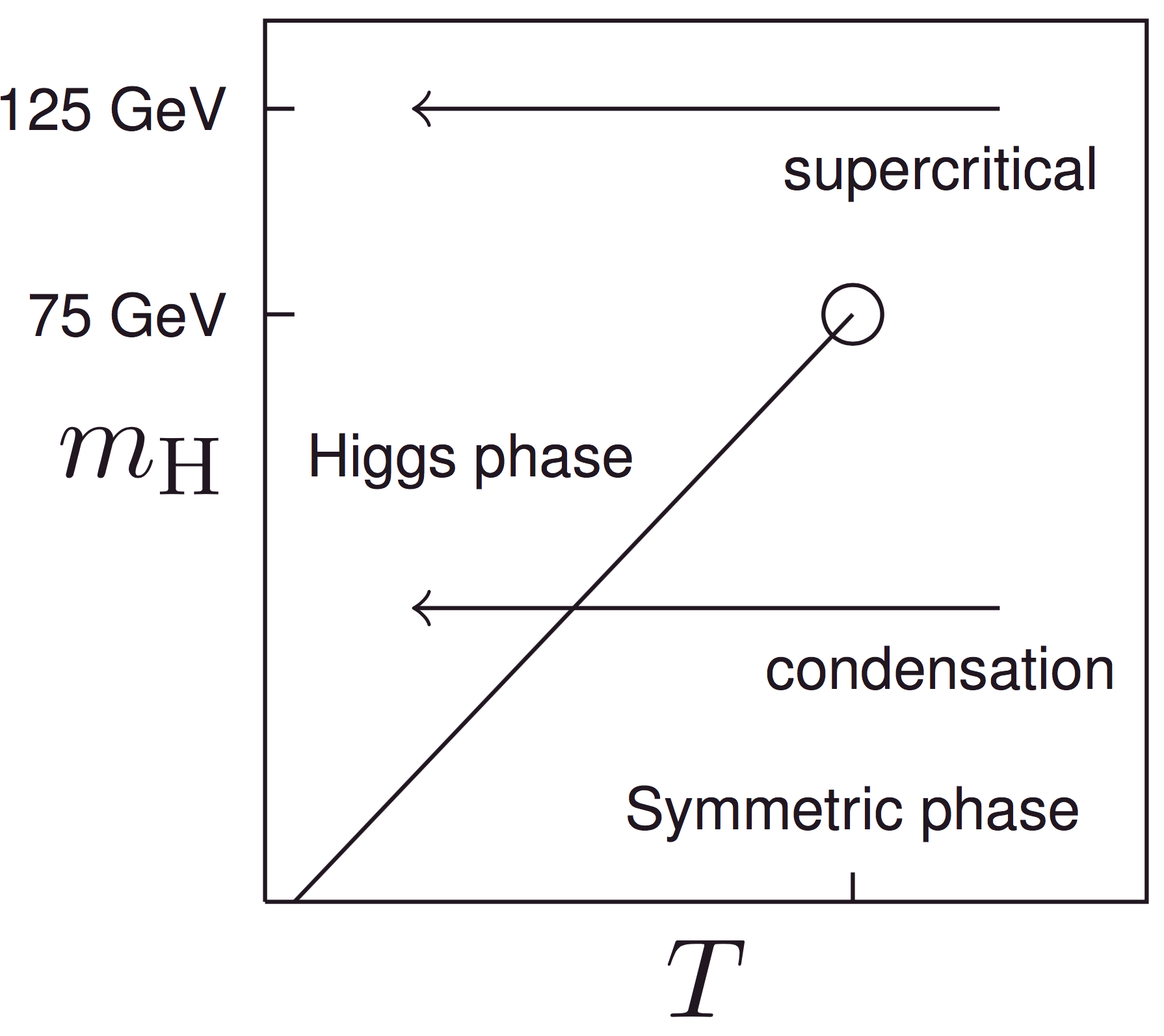
Thermal phase transitions
- Standard Model is a crossover
![]() Kajantie et al.; Karsch et al.; ...
Kajantie et al.; Karsch et al.; ...
- First order possible in extensions (xSM,
2HDM, ...)
Andersen et al.,
Kozaczuk et al., Carena et al.,
Bödeker et al., Damgaard et al.,
Ramsey-Musolf et al.,
Cline and Kainulainen,
...
- Baryogenesis?
- GW PS ⇔ model information?
- Standard Model is a crossover
![]() Kajantie et al.; Karsch et al.; ...
Kajantie et al.; Karsch et al.; ...
- First order possible in extensions (xSM,
2HDM, ...)
Andersen et al., Kozaczuk et al., Carena et al.,
Bödeker et al., Damgaard et al., Ramsey-Musolf et al.,
Cline and Kainulainen, ... - Baryogenesis?
- GW PS ⇔ model information?
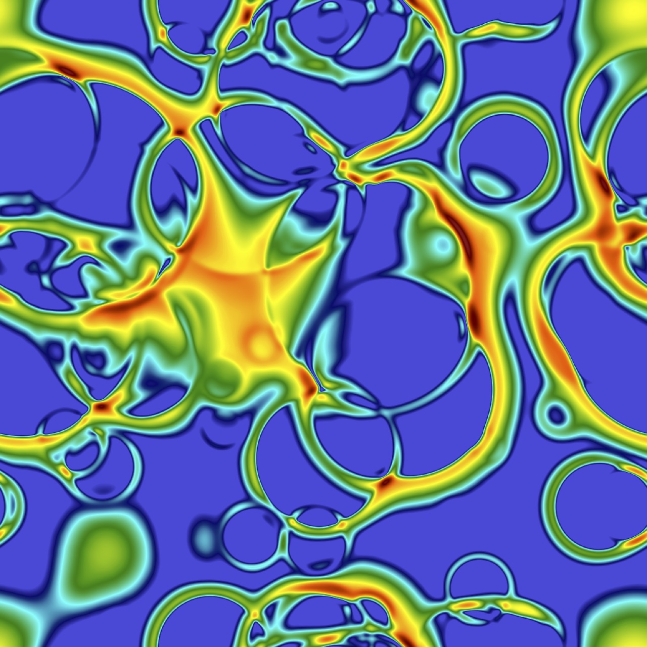
What the metric sees at a thermal phase transition
- Bubbles nucleate and expand, shocks form, then:
- $h^2 \Omega_\phi$: Bubbles + shocks collide - 'envelope phase'
- $h^2 \Omega_\text{sw}$: Sound waves set up - 'acoustic phase'
- $h^2 \Omega_\text{turb}$: [MHD] turbulence - 'turbulent phase'
- Sources add together to give observed GW power: $$ h^2 \Omega_\text{GW} \approx h^2 \Omega_\phi + h^2 \Omega_\text{sw} + h^2 \Omega_\text{turb}$$
- Equation of motion is (schematically)
Liu, McLerran and Turok; Prokopec and Moore $$ \partial_\mu \partial^\mu \phi + V_\text{eff}'(\phi,T) + \sum_{i} \frac{d m_i^2}{d \phi} \int \frac{\mathrm{d}^3 k}{(2\pi)^3 2 E_i} \delta f_i(\mathbf{k},\mathbf{x}) = 0$$- $V_\text{eff}'(\phi)$: gradient of finite-$T$ effective potential
- $\delta f_i(k,x)$: deviation from equilibrium phase space density of $i$th species
- $m_i$: effective mass of $i$th species:
- Leptons: $m^2 = y^2 \phi^2/2$
- Gauge bosons: $m^2 = g_w^2 \phi^2/4$
- Also Higgs and pseudo-Goldstone modes
Put another way:
$$ \overbrace{\partial_\mu T^{\mu\nu}}^\text{Force on $\phi$} - \overbrace{\int \frac{d^3 k}{(2\pi)^3} f(\mathbf{k}) F^\nu }^\text{Force on particles}= 0 $$This equation is the realisation of this idea:

Yet another interpretation:
$$ \overbrace{\partial_\mu T^{\mu\nu}}^\text{Field part} - \overbrace{\int \frac{d^3 k}{(2\pi)^3} f(\mathbf{k}) F^\nu }^\text{Fluid part}= 0 $$i.e.:
$$ \partial_\mu T^{\mu\nu}_\phi + \partial_\mu T^{\mu\nu}_\text{fluid} = 0 $$We will return to this later!
Envelope approximation

Envelope approximation
Kosowsky, Turner and Watkins; Kamionkowski, Kosowsky and Turner- Thin, hollow bubbles, no fluid
- Stress-energy tensor $\propto R^3$ on wall
- Solid angle: overlapping bubbles → GWs
- Simple power spectrum:
- One length scale (average radius $R_*$)
- Two power laws ($\omega^3$, $ \sim \omega^{-1}$)
- Amplitude
NB: Used to be applied to shock waves (fluid KE),
now only use for bubble wall (field gradient energy)
Envelope approximation
4-5 numbers parametrise the transition:
- $\alpha_{T_*}$, vacuum energy fraction
- $v_\mathrm{w}$, bubble wall speed
- $\kappa_\phi$, conversion 'efficiency' into gradient energy $(\nabla \phi)^2$
- Transition rate:
- $H_*$, Hubble rate at transition
- $\beta$, bubble nucleation rate
[only matters for near-vacuum/runaway transitions]
Envelope approximation
Coupled field and fluid system
Ignatius, Kajantie, Kurki-Suonio and Laine- Scalar $\phi$ and ideal fluid $u^\mu$:
- Split stress-energy tensor $T^{\mu\nu}$ into field and fluid bits $$\partial_\mu T^{\mu\nu} = \partial_\mu (T^{\mu\nu}_\phi + T^{\mu\nu}_\text{fluid}) = 0$$
- Parameter $\eta$ sets the scale of friction due to plasma $$\partial_\mu T^{\mu\nu}_\phi = \tilde \eta \frac{\phi^2}{T} u^\mu \partial_\mu \phi \partial^\nu \phi \quad \partial_\mu T^{\mu\nu}_\text{fluid} = - \tilde \eta \frac{\phi^2}{T} u^\mu \partial_\mu \phi \partial^\nu \phi $$
- $V(\phi,T)$ is a 'toy' potential tuned to give latent heat $\mathcal{L}$
- $\beta$ ↔ number of bubbles; $\alpha_{T_*}$ ↔ $\mathcal{L}$, $v_\text{wall}$ ↔ $\tilde \eta$
Begin in spherical coordinates:
what sort of solutions does this system have?
Velocity profile development: small $\tilde \eta$ ⇒ detonation (supersonic wall)
Velocity profile development: large $\tilde \eta$ ⇒ deflagration (subsonic wall)
$v_\mathrm{w}$ as a function of $\tilde \eta$
Cutting [Masters dissertation]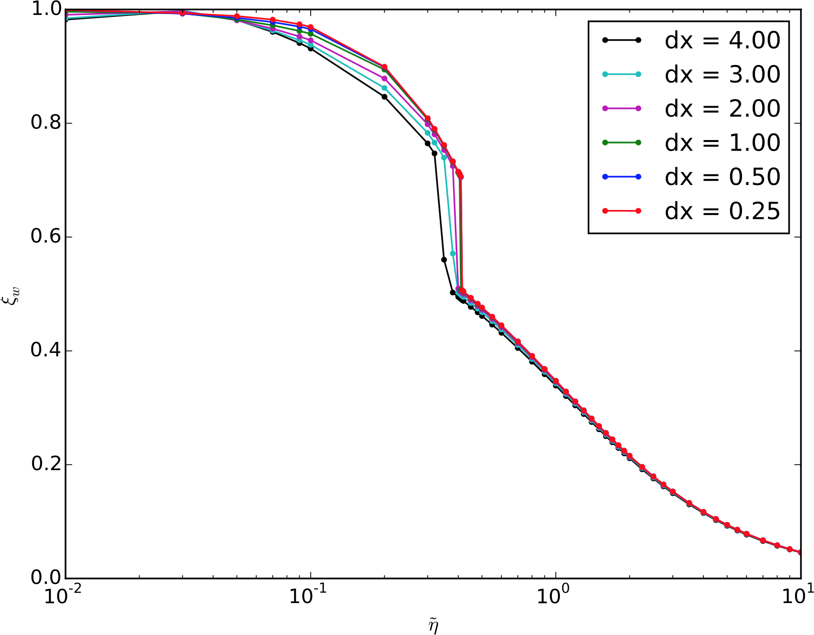
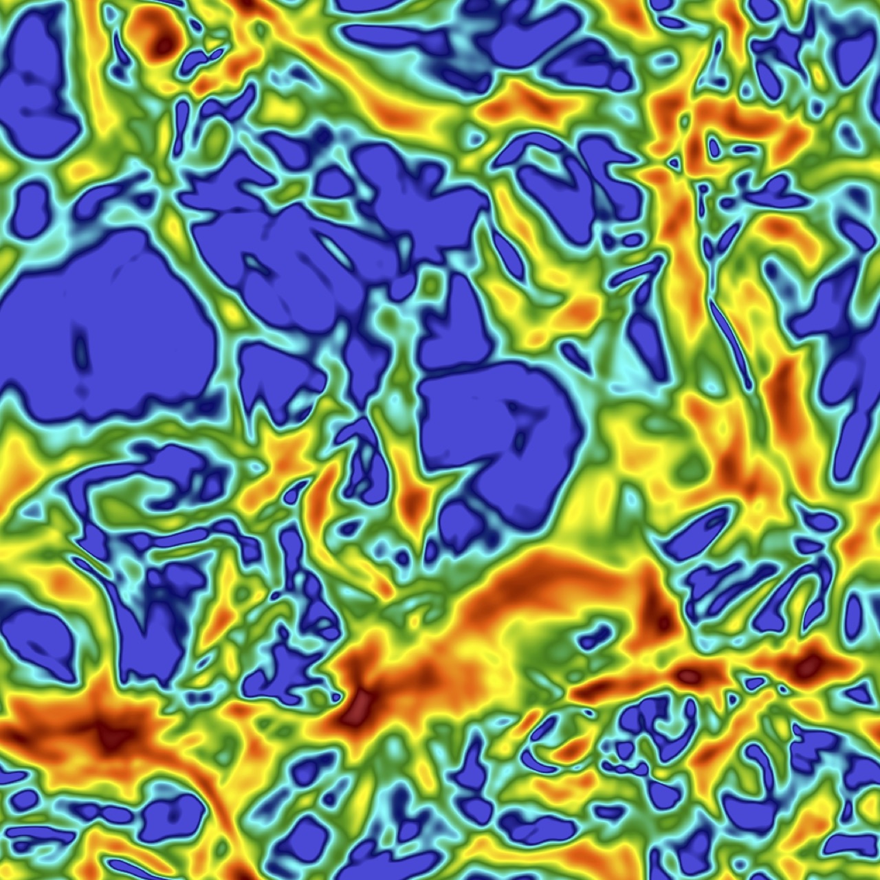
Simulation slice example
Velocity power spectra and power laws
Fast deflagration
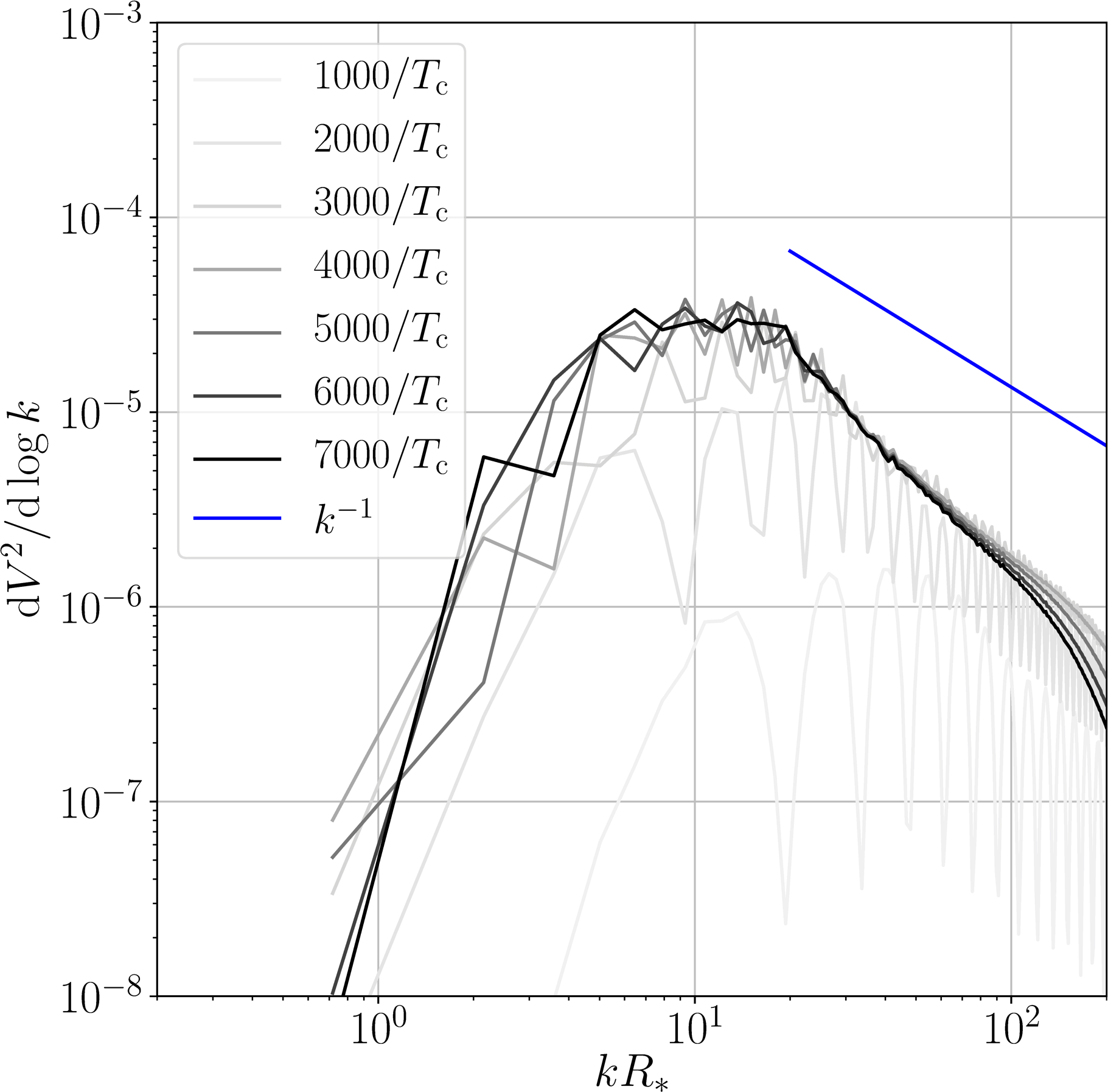
Detonation
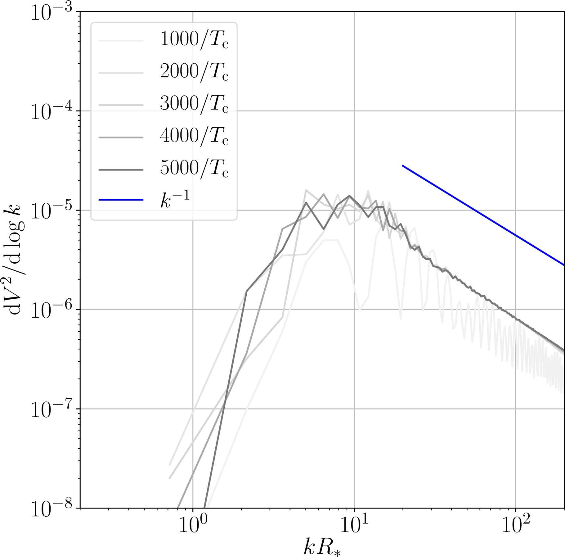
- Weak transition: $\alpha_{T_*} =0.01$
- Power law behaviour above peak is between $k^{-2}$ and $k^{-1}$
- “Ringing” due to simultaneous nucleation, unimportant
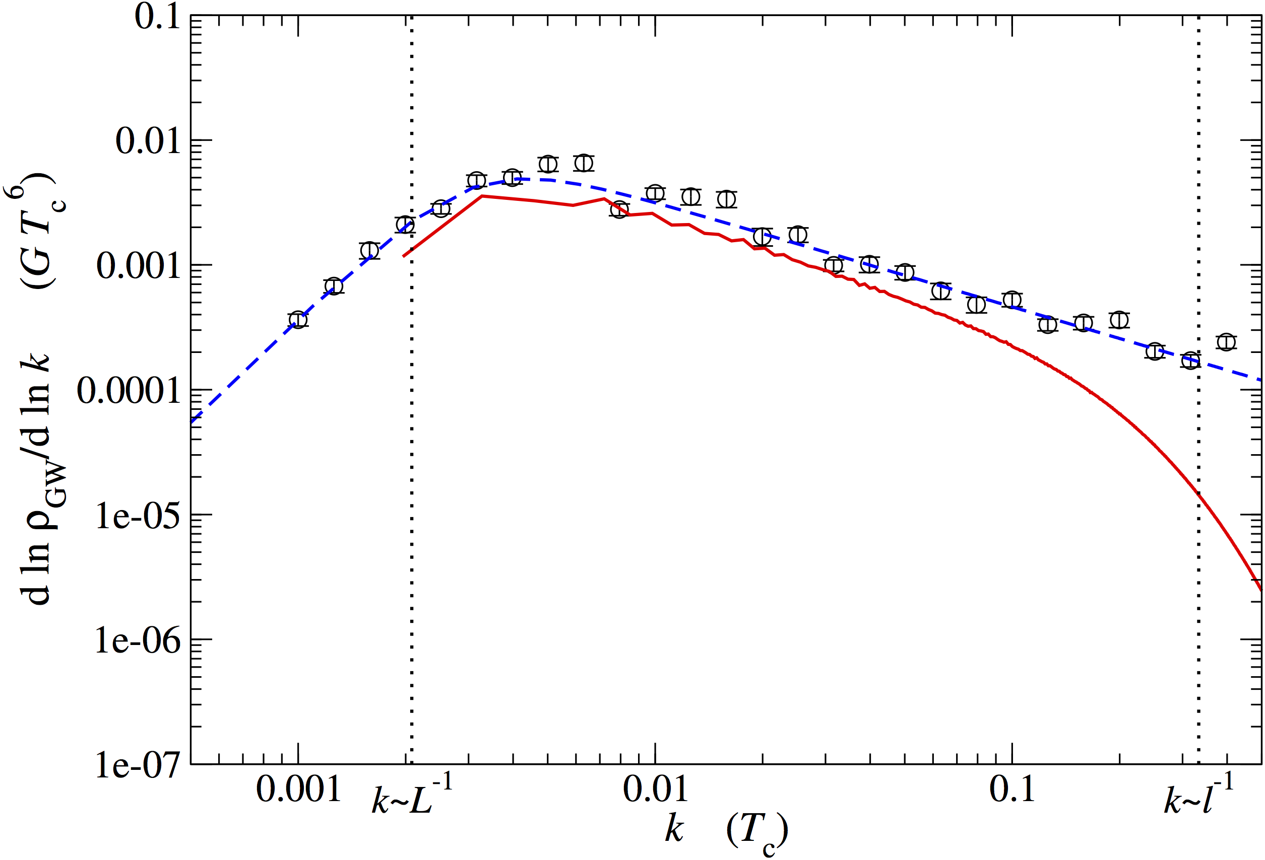
GW power spectra and power laws
Fast deflagration
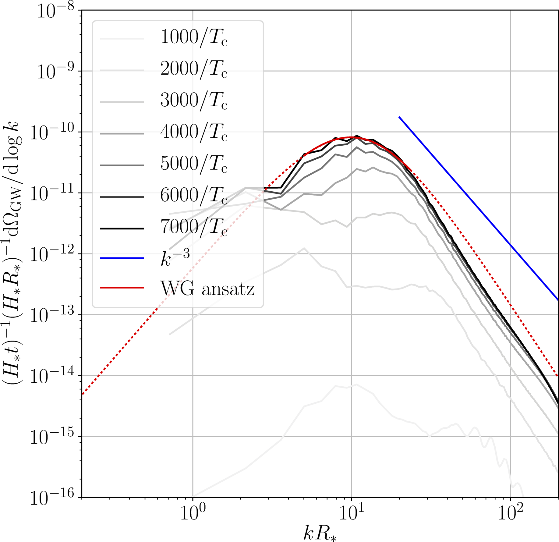
Detonation
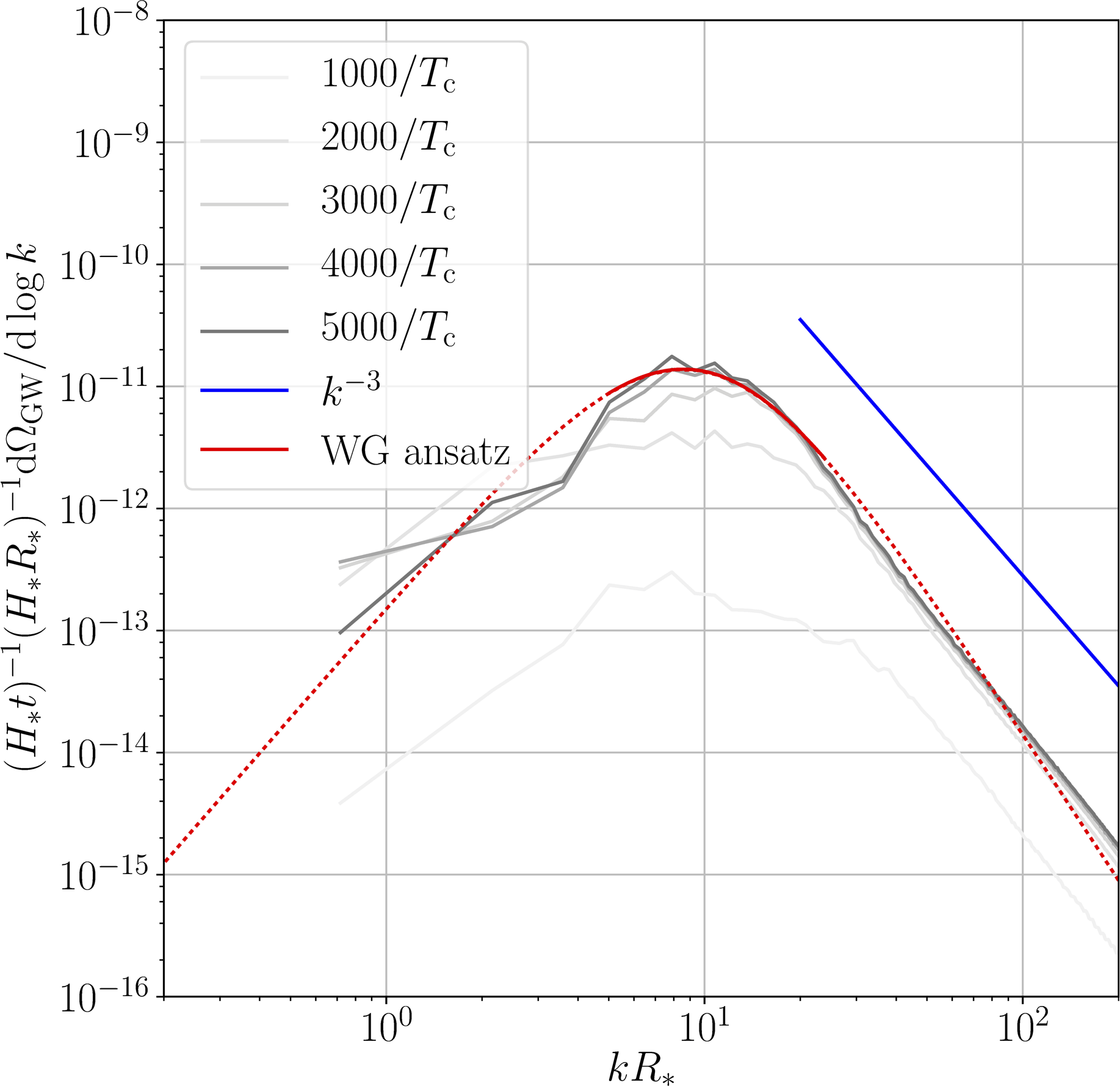
- Causal $k^3$ at low $k$, approximate $k^{-3}$ or $k^{-4}$ at high $k$
- Curves scaled by $t$: source until turbulence/expansion
→ power law ansatz for $h^2 \Omega_\text{sw}$
Transverse versus longitudinal modes – turbulence?
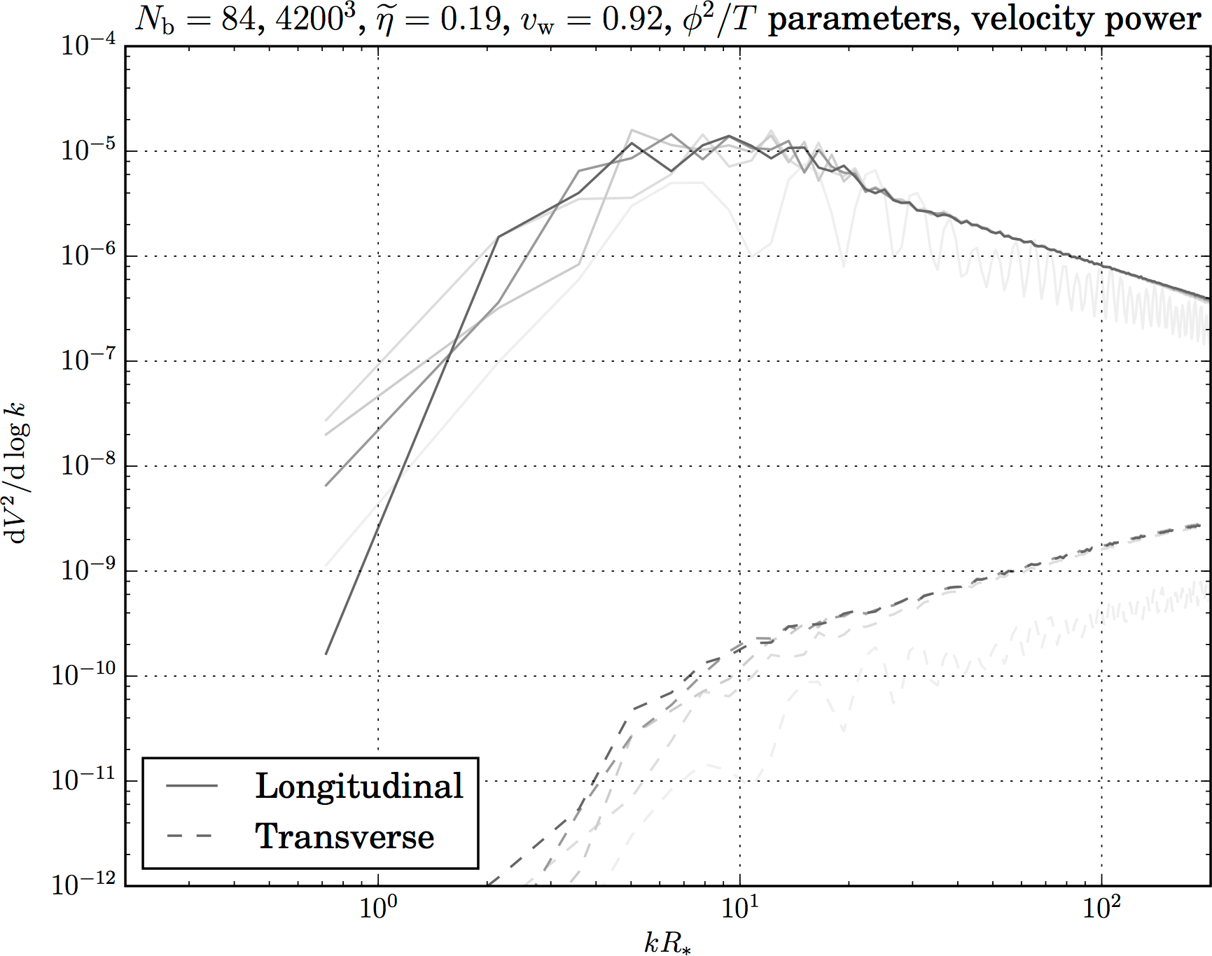
- Short simulation; weak transition (small $\alpha$): linear; most power in longitudinal modes ⇒ acoustic waves, turbulent
- Turbulence requires longer timescales $R_*/\overline{U}_\mathrm{f}$
- Plenty of theoretical results, use those instead
Kahniashvili et al.; Caprini, Durrer and Servant; Pen and Turok; ...
→ power law ansatz for $h^2 \Omega_\text{turb}$
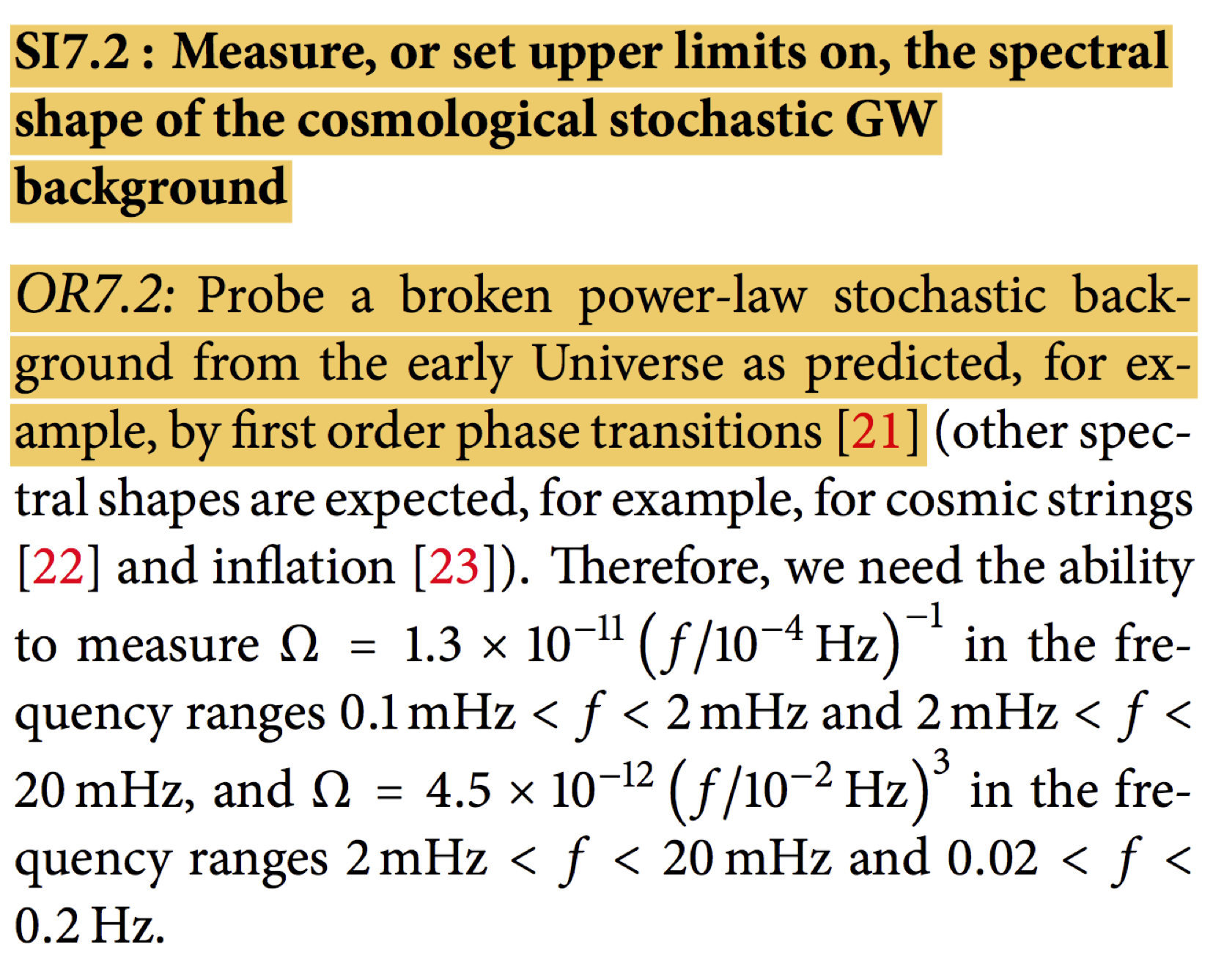
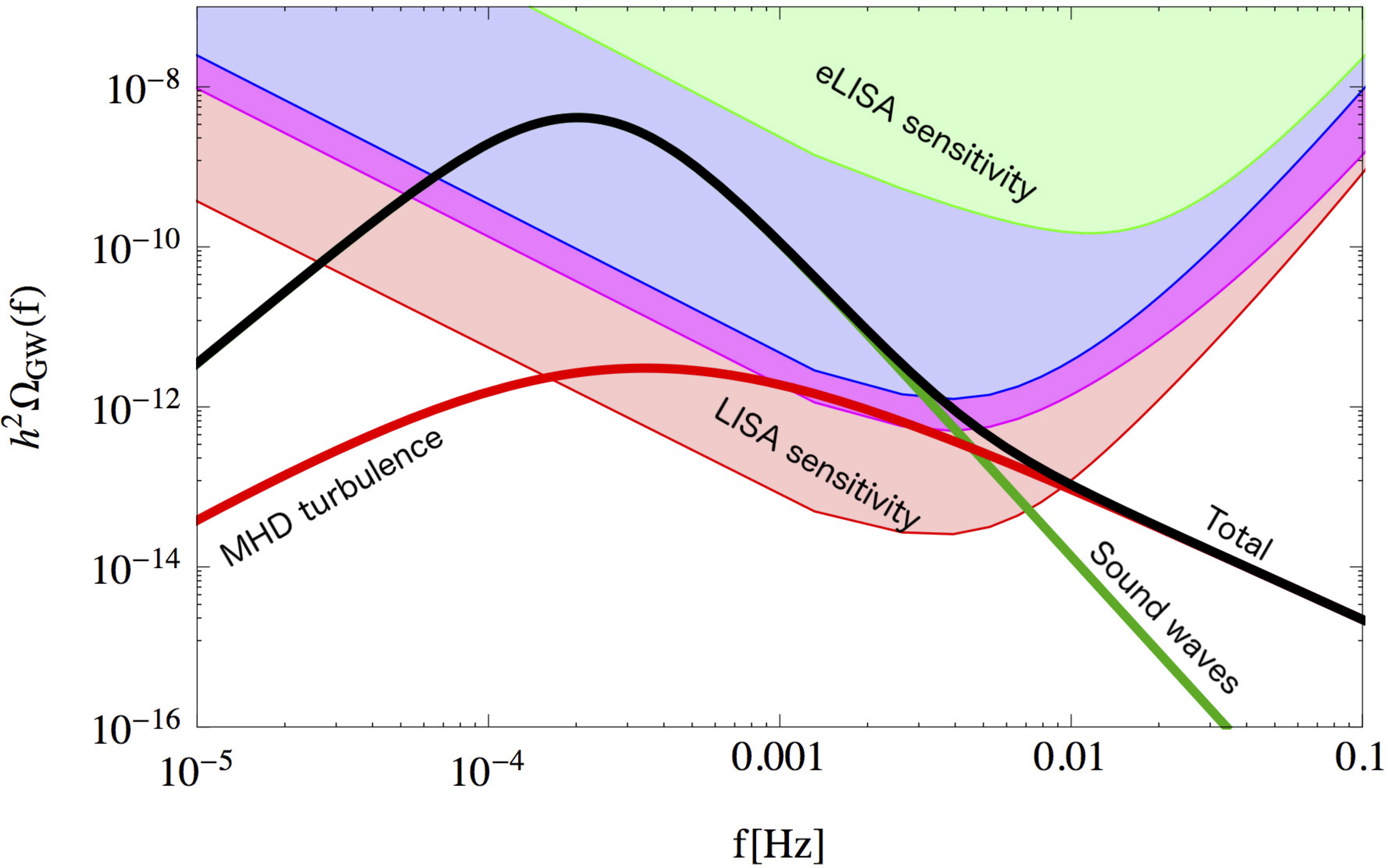
Putting it all together - $h^2 \Omega_\text{gw}$ arXiv:1512.06239
- Three sources, $\approx$ $h^2\Omega_\phi$, $h^2\Omega_\text{sw}$, $h^2 \Omega_\text{turb}$
- Know their dependence on $T_*$, $\alpha_T$,
$v_\mathrm{w}$, $\beta$
Espinosa, Konstandin, No, Servant - Know these for any given model, predict the signal...
(example, $T_* = 100 \mathrm{GeV}$, $\alpha_{T_*} =
0.5$, $v_\mathrm{w} =0.95$, $\beta/H_* = 10$)
Putting it all together - physical models to GW power spectra
Model ⟶ ($T_*$, $\alpha_{T_*}$, $v_\mathrm{w}$, $\beta$) ⟶ this plot
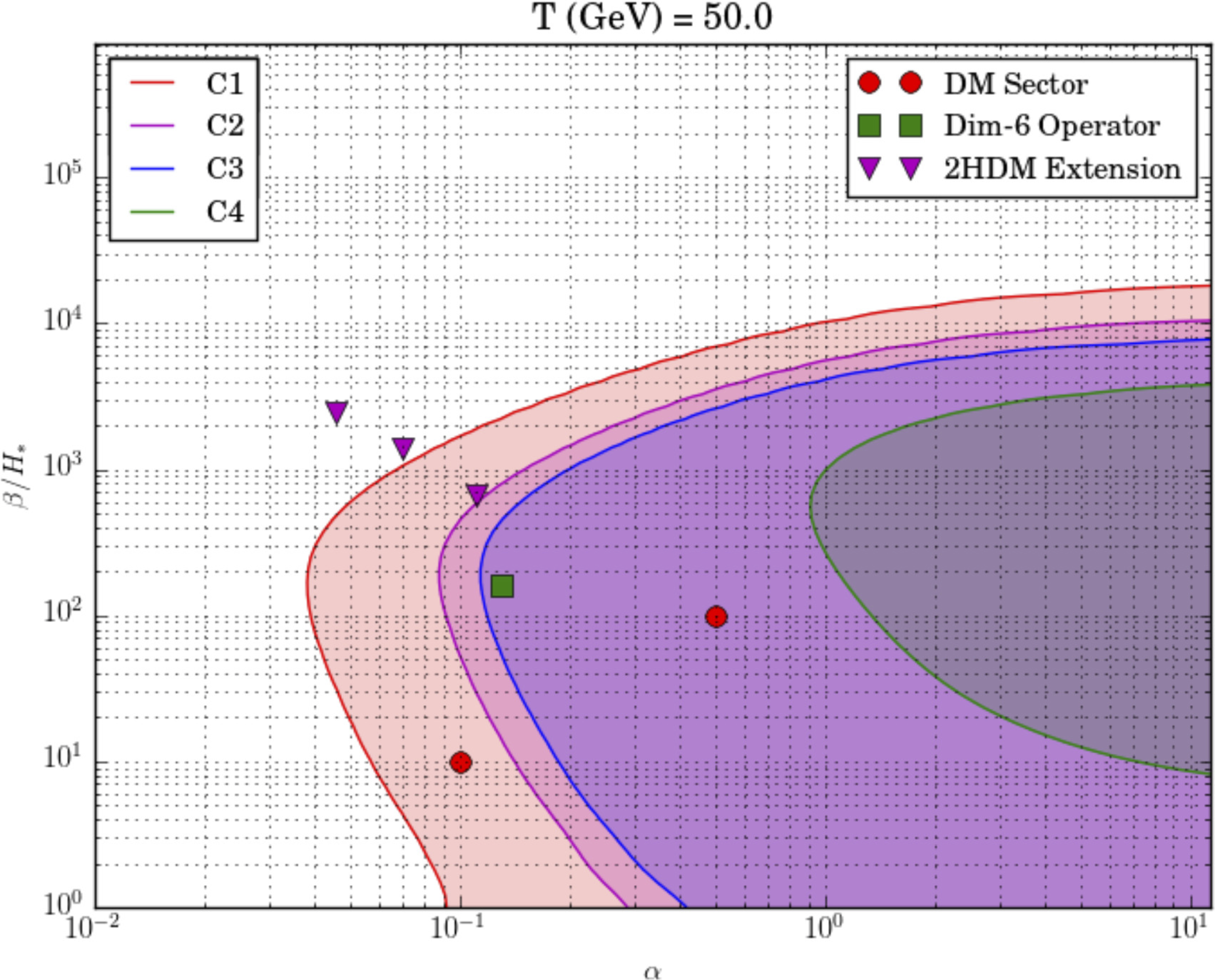
... which tells you if it is detectable by LISA (see arXiv:1512.06239)
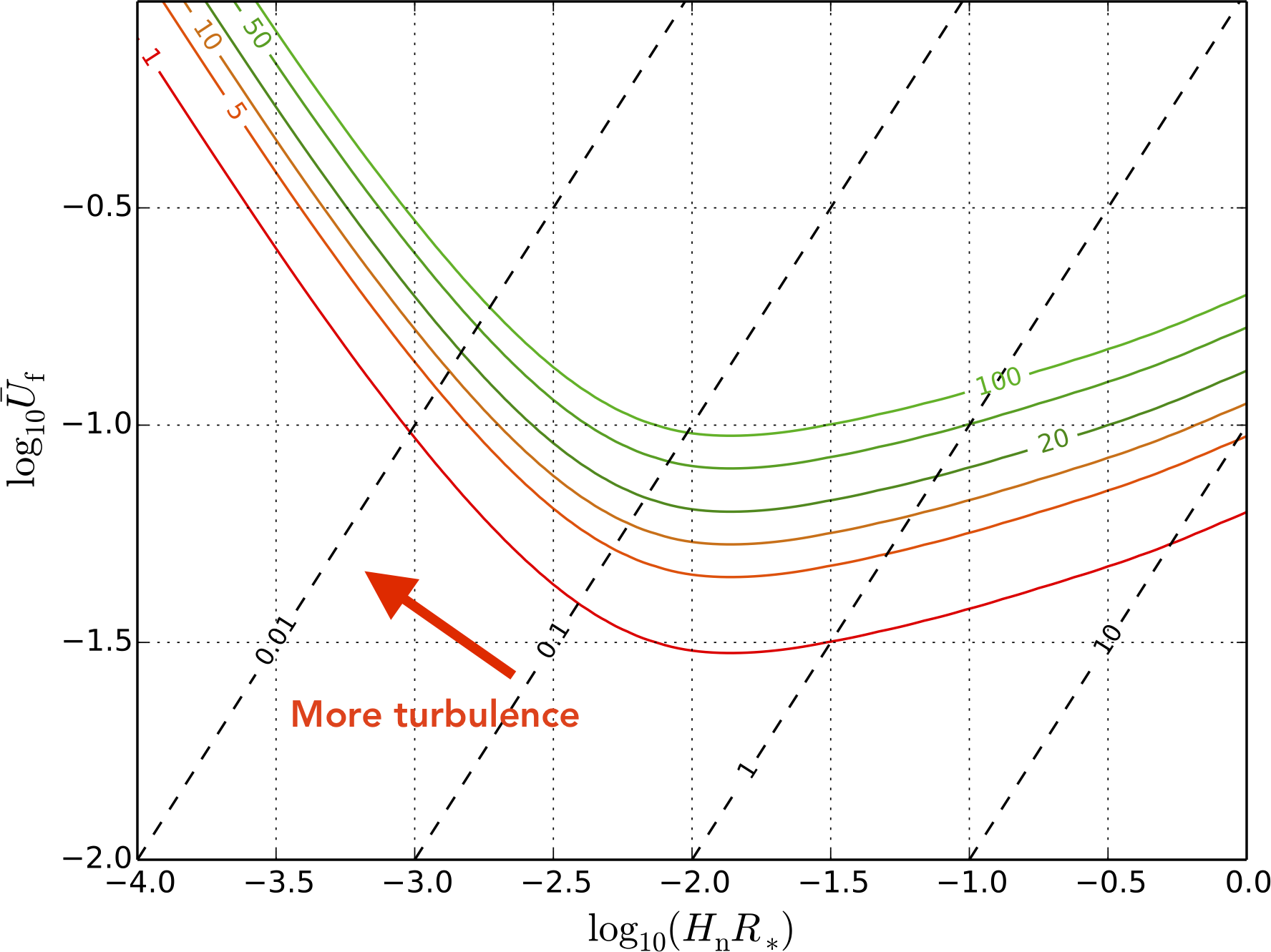
Detectability from acoustic waves alone
- In many cases, sound waves dominant
- Parametrise by RMS fluid velocity $\overline{U}_\mathrm{f}$ and bubble radius $R_*$ (quite easily obtained Espinosa, Konstandin, No and Servant)
Sensitivity plot:
The pipeline
- Choose your model
(e.g. SM, xSM, 2HDM, ...) - Dim. red. model Kajantie et al.
- Phase diagram ($\alpha_{T_*}$, $T_*$);
lattice: Kajantie et al. - Nucleation rate ($\beta$);
lattice: Moore and Rummukainen - Wall velocities ($v_\text{wall}$)
Moore and Prokopec; Kozaczuk - GW power spectrum $\Omega_\mathrm{gw}$
- Sphaleron rate
Very leaky, even for SM!
Questions, requests or demands...
- Turbulence
- MHD or no MHD?
- Timescales $H_* R_*/\overline{U}_\mathrm{f} \sim 1$, sound waves and turbulence?
- More simulations needed?
- Interaction with baryogenesis
- Competing wall velocity dependence of BG and GWs?
- Sphaleron rates in extended models?
- The best possible determinations for xSM, 2HDM,
$\Sigma$SM, ...
- What is the phase diagram?
- Nonperturbative nucleation rates?